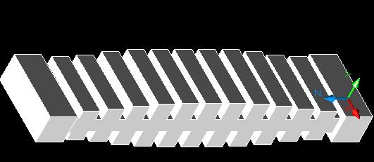
The main application of transmit-reject filters is to isolate the receiving channel from the transmitting channel. Due to the fact that there are different radio systems, the frequency ranges of the receiving and transmitting channels (possibli including multiple carriers) can be both close or significantly distant from each other. Because of this, the implementation of such a filter (we are considering microwave bands and only waveguide filters here) can be very different. In this case (Ka-band satellite links), when the frequencies of the downlink (18-21 GHz) are lower than the frequencies of the uplink (29.5-30 GHz) and when there is a significant distance between them, a corrugated waveguide low-pass filter can be the optimal technical solution. It should also be noted that in this case, rejection of the harmonics and other high-frequency interference is not required by specification. As a result, this greatly simplifies the design as it requires fewer corrugations. However, as it can be seen from the characteristics, the stop-band is still much wider than being required.

This filter has been requested for a VSAT system, designed using a "WR-Connect" (original Windows version), implemented in a single assembly with OMT and (supposedly) is still in service today.